Mars 2020

If you'd told me twenty years ago that I'd one day make a map of Mars compiled from images taken from my own back garden, I wouldn't have believed you. Even six years ago - the last time I had a good look at Mars - I probably would have been doubtful. Back then I was using a 102 mm achromat, and while I was able to identify Syrtis Major and the polar cap through the eyepiece, seeing anything more than that was beyond my capabilities.

The 2018 Mars opposition took place a few months after I got my 254 mm reflector (an Orion XT10 Plus), but an unfavorable southerly declination and a global dust storm meant I couldn't see much more than a shimmering yellow blob (albeit an impressively large blob).

As you've probably noticed, this year's opposition has been much more favourable for northern hemisphere observers. I started taking test images in early September (using a Tele Vue 2.5x Powermate to boost the XT10's focal length to 3,000 mm), and it was while experimenting with my ZWO ASI120MM Mini camera that I had my first stroke of luck. I bought this camera to use for autoguiding during long-exposure astrophotography, but it also functions well as a highly sensitive monochrome planetary imager, capable of capturing significantly finer detail than my Canon 80D DSLR. By sheer coincidence (I didn't plan it that way), the two cameras have almost exactly the same pixel size, making it relatively easy for me to combine the monochrome and colour data in Photoshop, as shown below:

One downside of using the ASI120MM is the difficulty of getting your target planet to drift perfectly across that tiny 1.2 megapixel chip - and then repeating that feat multiple times (remember, I'm using an undriven Dobsonian). I don't recommend trying this yourself unless you have a very well aligned finderscope, preferably one with illuminated crosshairs. 

Another problem is that switching cameras (and their associated adaptors and software) can take several minutes - long enough for Mars to show an appreciable amount of rotation. One way round this is to capture your colour and monochrome data exactly 24 hours and 37 minutes (one Martian day) apart and hope that neither your sky nor the Martian sky clouds over in the meantime. Another, better solution is to sandwich your colour image set with two monochrome sets and use the WinJUPOS software to merge and derotate the monochrome data; aligning the "bread" with the "filling", so to speak.

I won't go through the laborious process of stacking and sharpening, then registering and merging the data in WinJUPOS and Photoshop, when perfectly good tutorials already exist online (see the links at the end of this post), but if you image Mars regularly over the course of several weeks, eventually you should get enough data to make a map like the one at the top of this post. A run of very poor weather through the middle of October meant my coverage of the region centred on 130 degrees longitude wasn't as good as I would have liked, but hey, in an English autumn you take what you can get. Admittedly, I probably could have done a better job of hiding the vertical seams between the different sections, but the end result was still better than anything I could have hoped to achieve when I embarked on this crazy project.

Another thing you can do in WinJUPOS is to wrap your carefully assembled map back onto a sphere and make a rotation video, as shown below:

Seeing Mars

This autumn wasn't purely devoted to imaging; I also took time to observe Mars through the XT10, switching between the following magnifications depending on what the atmospheric seeing would allow:

171x (7mm DeLite)

240x (5mm Nagler)

333x (9mm Nagler + 2.5x Powermate)

428x (7mm DeLite + 2.5x Powermate)

And here's my second stroke of luck: while browsing the Cloudy Nights forums, I learned that the Baader Contrast Booster filter (which I bought years ago for the refractor) is also very good at enhancing detail on Mars. It also has a warming effect: without the filter Mars has a pale butterscotch hue; with the filter in place it appears more tangerine in colour, closer to the Mars you typically see in photos.

A stubbornly persistent jet stream meant that the moments of truly excellent seeing I was hoping for were limited to a few fleeting seconds at best (fine for imaging, but not so great for observing), but for the most part the visible detail approximated that shown in the first Canon 80D image above.

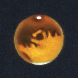
Here's a pastel sketch of Mars as it appeared on the night of 21 to 22 October, with Solis Lacus, the "eye" of Mars, at centre stage. This view shows south at the top, as it appears in a Newtonian reflector.

It's important to note that I've greatly exaggerated the contrast in this sketch; even with the Baader filter in place the differences between the dusky southern highlands and the lighter northern plains are subtle. It's also worth pointing out that the detail shown here doesn't present itself all at once. The first thing you notice when looking through the eyepiece is that Mars is very small and very bright (even at the highest magnifications). After a few seconds, as your eyes adjust, the tiny but brilliant South Polar Cap (SPC) should become apparent - although, at time of writing, it has shrunk to about half the size shown above. As most astronomers know, the art of seeing - and I mean really seeing as opposed to just looking - is a skill that requires many nights of practice: the first time I looked at this region of Mars (in September), I could immediately tell that the southern hemisphere was darker than the north, but it took a few minutes before I realised that Solis Lacus was staring right back at me. When I looked at it again in October, it was obvious straight away. Over the last couple of months I've been lucky enough to see all the major albedo features shown on the map at the top of this post, as well as the hazy North Polar Hood - its subtle blue tinge contrasting with the intense whiteness of the SPC (these cooler hues are best seen without the Baader filter). However, there is always room for improvement; the finer details revealed by the ASI120MM have eluded me so far: I haven't seen Olympus Mons (yet) which is why it wasn't included on the sketch.

At time of writing Earth is now racing ahead of Mars, but the red planet will remain a fixture in the evening sky for a few months to come. For the next opposition in 2022 it will occupy the winter constellation of Taurus, but its apparent size will max out at a more modest 17 arcseconds (compared to this October's maximum of 22.4 arcseconds). In the meantime there's plenty to look forward to with three new missions due to arrive at Mars in February 2021, aiming to advance our understanding of this enigmatic planet:

Hope Orbiter (United Arab Emirates)

Tianwen-1 (China), including an orbiter, lander and rover

Mars 2020 (USA), including the Perseverance rover and the Ingenuity helicopter drone

Links

Which side of Mars will I see tonight - Ade Ashford | British Astronomical Association

How to capture scientific images of Mars - Pete Lawrence | Sky at Night Magazine

Use WinJUPOS to derotate your planetary images - Martin Lewis | Sky at Night Magazine

Imaging the planet Mars - Roger Hutchinson

WinJUPOS download site

A Very Photogenic Comet

"Comets are like cats: they have tails, and they do precisely what they want." - David H. Levy

I must admit, when I first heard that comet C/2020 F3 (NEOWISE) was on course to reach naked-eye visibility, my initial reaction was one of mild scepticism. After all, similar predictions had been made about comet C/2019 Y4 ATLAS (which promptly disintegrated) and comet C/2020 F8 SWAN (which also fizzled out). However, NEOWISE didn't just live up to expectations, it surpassed them - becoming certainly the best comet I've seen since Hyakutake and Hale-Bopp, the two Great Comets of the 90s.

Bright though it is however, NEOWISE (named after the space telescope that discovered it) is by no means a Great Comet like those two. Nor is it the first significant comet of the digital age (that honour must go to the spectacular Comet C/2006 P1 McNaught), but - due to its favourable placing for observers in the northern hemisphere - it's likely to become the most photographed comet in history (at least until the next bright one comes along). This is the fifth comet I've pointed a camera at, and it's easily the most photogenic, even if it did require me to leave the house at some very unsociable hours.

Comet NEOWISE should remain visible for the rest of the month, although it will - barring outbursts - become progressively fainter. At time of writing NEOWISE can be found in the late evening sky below Ursa Major (see the links at the end of this post for finder charts). You don't need a telescope to spot it; if your sky is dark enough it should be visible to the naked eye, and a modest pair of binoculars will give a really good view.

You don't necessarily need a long lens either if you want to try and photograph it (the image at the top of this post was taken with a standard 50mm prime). However, you will need a tripod and some means of operating the shutter without touching the camera (either a timer delay or a cable release). As I was shooting at a high ISO I also stacked multiple images and subtracted dark frames to further improve the signal-to-noise ratio. Here's another one taken at 400mm, showing the characteristic golden dust tail:

It's worth making the effort to see Comet NEOWISE at least once before it's gone; after all, it won't return to the inner solar system for nearly 7,000 years.

Links:
How to see Comet NEOWISE over the coming nights (Sky at Night Magazine)
Comet NEOWISE dazzles at dusk (Sky & Telescope)

Siril: Old Data, New Tricks

Siril (https://www.siril.org/) is a (relatively) new freeware program for stacking and processing astronomical images. I've been using it for a couple of months now and although I'm still very much in the learning curve stage, I'm already finding it to be significantly better than its freeware rivals.

Shown below is a crop of an image of Messier 33 (the Triangulum Galaxy), compiled from two hours of data and processed in Siril. Move your cursor over the image to see my previous attempt at processing the same data in DeepSkyStacker (DSS).

 

(The full-size version of this image is available on my Flickr page.) As you can see, the improvement is quite dramatic, particularly in the faint outer spiral arms where a wealth of extra detail is revealed. Siril also does a much better job of preserving the colour information from the original raw files. If you've used DSS to stack raw files you may have noticed that the colours come out very muted (as explained in this informative thread on Cloudy Nights). Prior to using Siril, my workaround was to stack the data again in Sequator (effectively using that as an RGB layer and the DSS output as a luminance layer), which always seemed an unnecessarily convoluted way of going about things considering I'm not a dedicated astro-imager.

So how does it work? Video tutorials and manuals are available online, but here's a quick step-by-step guide (applicable to version 0.9.12) to get you started.

When you install Siril it will create four sub-folders in your Pictures directory, one each for light frames, dark frames, flats and bias frames. Make sure your raw files are in the appropriate folders and from the Siril menu select Scripts > DSLR_preprocessing. (Variant scripts are available if you don't collect darks or flats or some other combination.) You'll need a generous amount of disk space because Siril will create individual fit files for every single raw file - but you can safely delete these once the process is completed (just don't delete your raws!).

A live Output Log window shows the script's progress. It takes between 30 and 60 minutes to run on my laptop (about the same time as DeepSkyStacker).

Upon completion, the script will save a file called result.fit in your Pictures folder. This is the linear 32-bit file (if you've used DeepSkyStacker it's equivalent to the autosave.tif file) and it will look excessively dark because most of the useful data is bunched over to the far left of the histogram. At this point I would recommend renaming the result.fit file to something more meaningful and keeping it somewhere safe, just in case you later find you've overcooked your histogram-stretching and want to have another crack at it.

The image will require a bit of work before it's ready for processing in Photoshop or whatever your preferred image editor is. Fortunately Siril has all the tools you need under the Image Processing menu.

First, change the Display Mode dropdown at the bottom of the image screen from Linear to AutoStretch or Histogram to get a better sense of the quality of your data. The Histogram display mode (like Equalize in Photoshop) is useful for showing the dark boundaries caused by tracking drift over the course of the imaging session. Draw a box on the image to exclude these dark areas and then right-click and select Crop. (You can always carry out a more precise crop later on in Photoshop.)

Siril image window in AutoStretch display mode

The Histogram preview will also show if there's a light pollution gradient in your image. Remove this by selecting Image Processing > Background Extraction. You can select background samples manually or click on the Generate button to have Siril select them automatically. Then click Apply to correct the image.

Change the display mode back to AutoStretch. The RGB image will now likely have a strong green tint. Remove this by selecting Image Processing > Remove Green Noise... and click on Apply.

Any remaining colour bias can be corrected by selecting Image Processing > Colour Calibration > Colour Calibration. Here you'll need to select an empty part of the background before clicking on Use Current Selection and then Background Neutralisation. Then repeat the process for the White Reference section (this time drawing a box around the brightest part of the image).

Now you're ready to begin stretching the image. Change the preview mode back to Linear and select Image Processing > Histogram Transformation. You may have to magnify the histogram to see where the data is. Drag the Midtones slider to the left and the Shadows slider to the right (making sure you don't clip your data). Click on Apply to apply the transformation. As you're probably aware, histogram stretching is an iterative process and will need to be repeated several times to get the desired result. (Hopefully the preview display modes will have given you an idea of where the data ends in your image and where the noise begins.) For images with complex dynamic ranges (such as the Orion Nebula) you may have to create two separate stretched images (one for the core and one for the fainter outer regions, and carefully layer them together in Photoshop).

Siril histogram window

Other functions on the image processing menu which may be useful at this stage include Colour Saturation (for boosting the colour), Median Filter (for reducing noise), and Deconvolution (for sharpening) - although the latter does take a long time to run. Otherwise, you can export the image as a 16-bit TIF by selecting File > Save as... ready for finishing off in Photoshop or your image editor of choice.

Here's one more example, showing Messier 27 (the Dumbbell Nebula) in Vulpecula. Again, move your cursor over the image to see the original (DSS) version.

 

(A larger crop of this image is available on my Flickr page.) Detail-wise, the differences are subtle (because M27 is one of the brighter DSOs), but look closer and you'll see that the fainter outer regions of the nebula stand out more clearly in the Siril version. I also prefer the rich blue colour in the newer version. Which one do you prefer?